(Pseudo) Differentiable JPEG - Computing Gradients from Noise
In the previous post, we explored how deep learning can be used for image steganography. But as cool as that sounds, it turns out to be pretty impractical - no support for lossy image compression and easily fooled by adversarial attacks, even though it can handle a hefty 24 bits per pixel. So, after all that training, why can’t this neural network figure out image compression? Simply put, the decoder was not trained to recognize image compression in the first place. As you can see, deep learning models can be super sensitive to the data they’re trained on. So, if the training data doesn’t reflect real-world scenarios like random noise or image compression, there’s no way the neural net can be ready for such situations.
The Problem
So, let’s circle back to the code we implemented earlier. When we tested the model, we used something like this:
cover   = decode_img(COVER_IMG_PATH)
payload = decode_img(PAYLOAD_IMG_PATH)

steg_image    = encoder_model([cover,payload])
decoded_image = decoder_model(steg_image)
This gives us an output as follows:
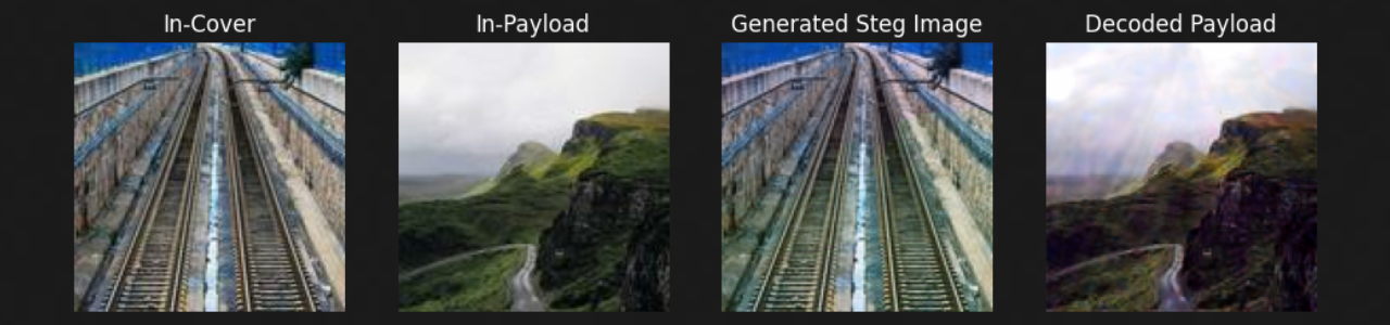
The generated steganographic container image looks pretty good, but the decoded payload image has some minor visual artifacts. We could improve this by training the model for more epochs and tweaking the value of the β parameter in the loss function. But here’s the thing: in the current implementation, the output of the encoder is fed directly into the decoder. In a real-life scenario, wouldn’t we be saving it to a file, transmitting it over some medium, and then reading it back from the file to decode it?
Hmm, let’s first try using a lossless image format like PNG. The encoder output gets saved as a PNG using Pillow, then it’s read back and fed into the decoder. The output pretty much stays the same as when we fed the encoder output directly into the decoder. Makes sense, right? The file format is lossless, after all. But what happens when we save it using a lossy file compression such as JPEG? Not everyone uses PNG, and most social media or messaging platforms like Instagram, Facebook, X (formerly Twitter), and WhatsApp uses lossy compression formats like JPEG or WebP to cut down on their web costs while handling images for millions of users.
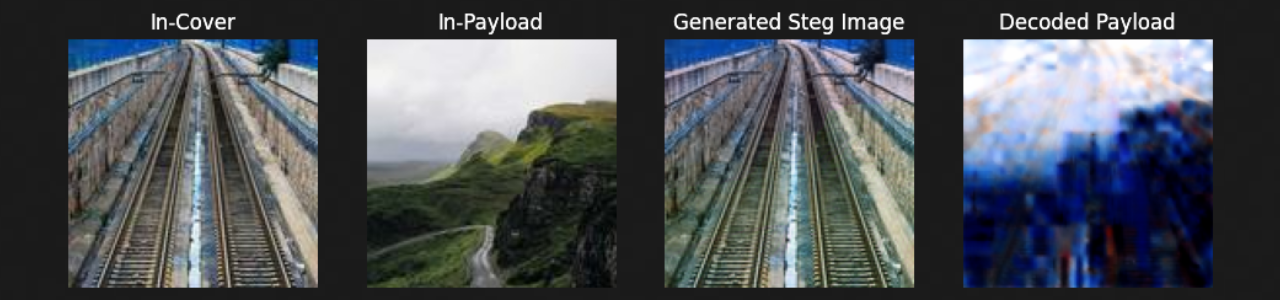
Instead of decoding an image of a winding mountain road, you get slapped in the face with a mess of blue blotches and patches. Clearly, our network hasn’t figured out how to handle lossy compression during training. So, how do we fix this? One common approach is to add a layer between the encoder and decoder. This layer tweaks the output from the encoder to simulate noise from factors like image compression and other sources, before sending it to the decoder during training.
The Issue with Image Compression
The problem with sticking an image compression layer in the middle of a neural network during training is the issue of differentiablity. In short most lossy image compression algorithms contain operators which aren’t differentiable. Now why is this an issue?
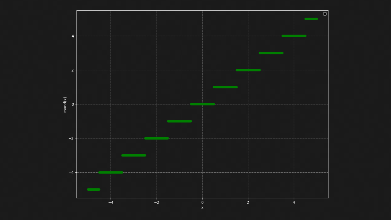
Neural networks update their weights during training using a technique known as Gradient Descent. The actual weight updates are informed by the gradients computed during backpropagation, where derivatives are used to calculate the gradient of the loss function with respect to each weight. Now, if we recall our high school math, we know that not all functions have derivatives. For a function to have a derivative, certain conditions are to be met such as continuity, presence of a limit, equality of limits, etc. Keeping this in mind, let’s turn our attention towards why image compression algorithms have an issue with computing derivatives.
Let’s take a quick look at the JPEG image encoding and decoding process. I won’t get into the exact details here, but in short, an image is JPEG encoded through a series of operations and then decoded using operations that are essentially the inverse of the encoding steps.
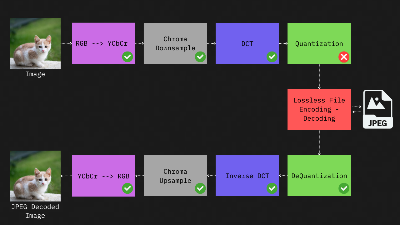
For a deeper dive into this process you can have at a look at this article. From the figure above, you’ll notice that almost every operation is differentiable (marked with a green check), except for the ‘quantization’ step. Here, values in the quantization table during the previous DCT operation are rounded to the nearest whole number based on the ‘q’ or ‘quality’ parameter. This rounding introduces a jump discontinuity, which makes it impossible to compute derivatives for this step. Most neural network libraries either throw an error or return a zero gradient when they encounter the round operation. The lossless file encoding-decoding operations are not considered as it’s basically an identity function.
The effect of getting zero gradients from the image compression layer during backpropagation is that the encoder network will always receive zero gradients, no matter what inputs or training examples are used. It’s like trying to guess what’s on the other side of a wall with no information — essentially, the encoder is left in the dark and has to make guesses.
A Pseudo-Differentiable Approach
In the paper titled Towards Robust Data Hiding Against (JPEG) Compression, Zhang et al. introduces a pseudo-differentiable approach that adds the true distortion of image compression as pseudo-noise to the original image. So what does this jargon mean? In section 3.3 of the paper, the author quotes as following:
Regardless of the attack type, the resulting effect is a distortion on the encoded image. Specifically, Gaussian noise is independent of the encoded image while the JPEG distortion can be seen as a pseudo-noise that is dependent on the encoded image.
In simple terms, the author views image compression as a process that results in the addition of distortion or noise to an input image. While Gaussian noise adds noise irrespective of the input image, JPEG or any image compression algorithm, adds noise that is specific to the characteristics of the image. If the addition of Gaussian noise to an image is considered differentiable (because adding a constant to a differentiable function maintains differentiability, and Gaussian noise acts as a random constant), then the addition of JPEG (pseudo) noise to an image can also be considered differentiable. So how do we compute this pseudo noise? The paper introduces an approach for computing pseudo noise as shown in the figure below.
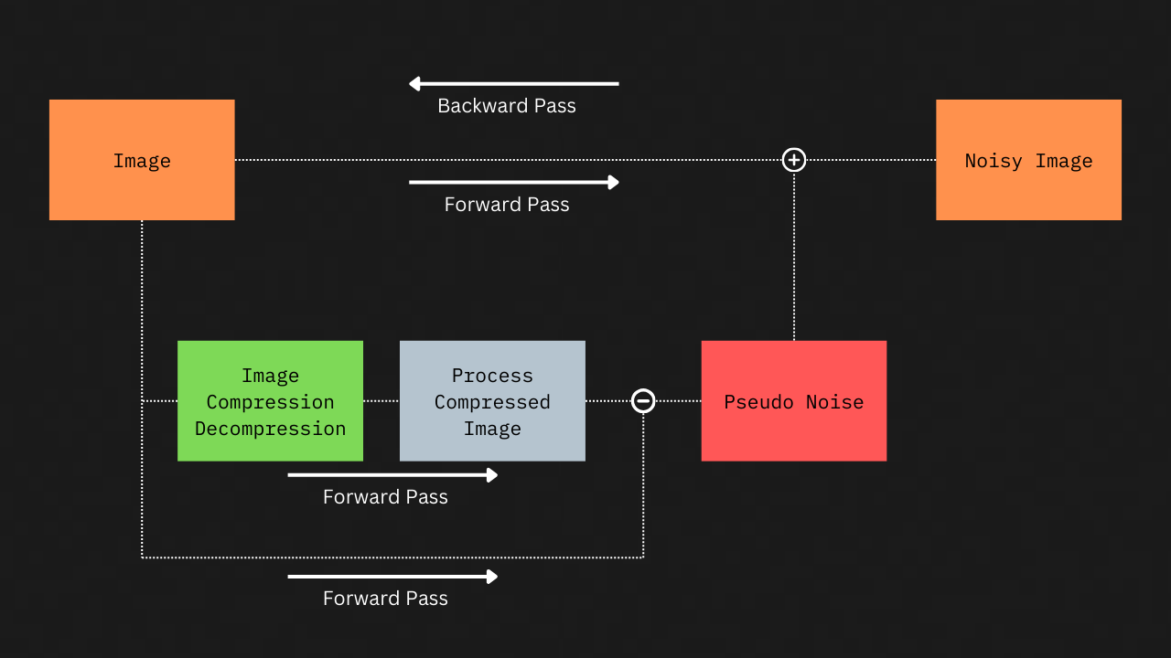
During the forward pass, operations are performed on both the image pathway and the pseudo-noise pathway. However, during backpropagation, gradients are computed only for the image pathway. Since the backward pass does not include the pseudo-noise path, the non-differentiability of JPEG compression does not cause the gradients passed to the encoder network to be zero.
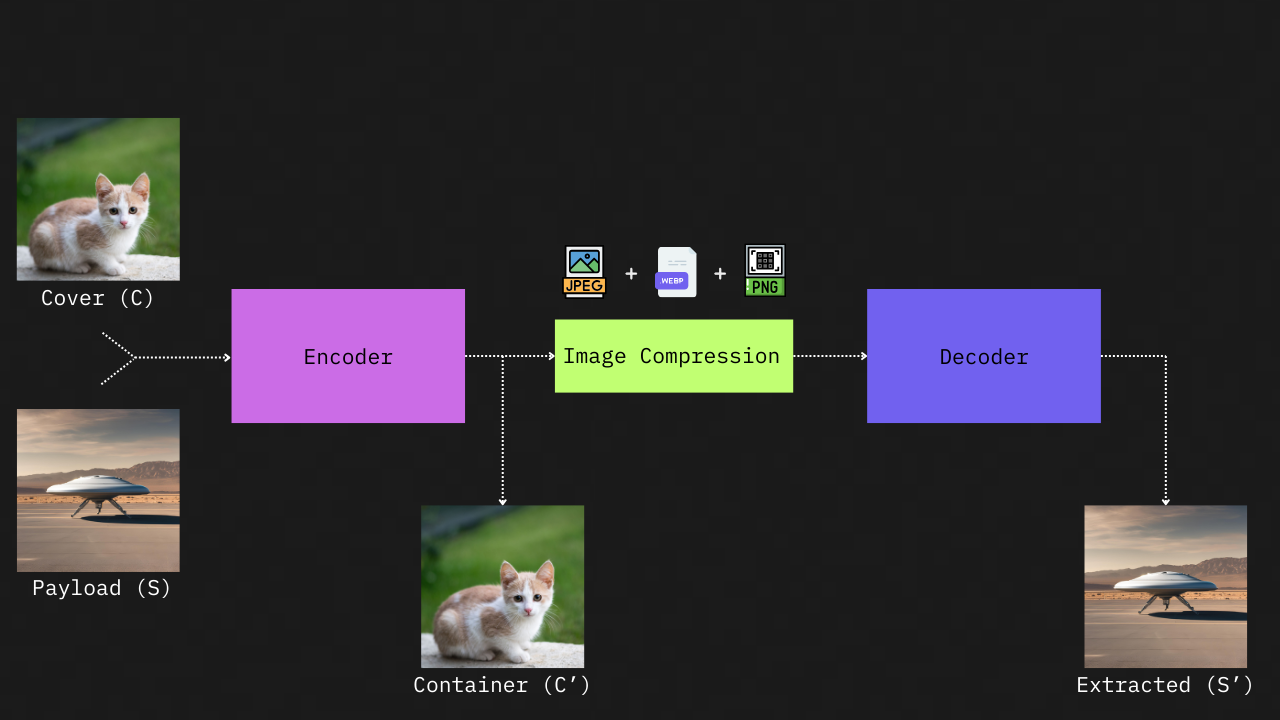
The beauty of this approach is that we are not limited to just JPEG. Any image compression algorithm - whether it’s JPEG, WebP or something new that comes up in the future could be added as a layer during neural network training.
For implementation you can check out the notebooks at github.com/Acedev003/Deep-Steganography.
Recent Alternatives?
While this pseudo-differentiable approach helps with a lot of our problems, it’s more of a hack than a real solution to true differentiable JPEG. The gradients here are entirely independent of the actual JPEG function and are computed just from residual noise. This can lead to issues if not handled carefully. For instance, while training a model with this approach, I found that the model became super sensitive to the specific implementation of the JPEG algorithm.
I initially used the ‘adjust_jpeg_quality’ function from tensorflow for the image compression layer. This worked fine with JPEG images compressed using TensorFlow’s function, but when I used images compressed with Pillow, the whole thing broke down. Same occurance when tried out with OpenCV. It turns out that even though the output was a JPEG file in all three cases, these libraries used slightly different implementations under the hood to generate jpeg images. This results in minute differences in the residual noise, which our overly sensitive model picked up on. I assume (emphasis on “assume” - I haven’t tested this yet) that if the model had knowledge of the specific operations involved in image compression encoding and decoding, this kind of oversensitivity to different JPEG implementations might not have occurred.
A more recent approach to attaining differentiable JPEG image compression is a paper titled Differentiable JPEG: The Devil is in the Details. This introduces differentiable clipping of both the codec image and the quantization table along with differentiable implementations of clipping and floor operators. A Straight-Through Estimator (STE) is also proposed to improve approximation performance. For more details and implementation code on this you can check out the following article.
References
-
Zhang, C., Karjauv, A., Benz, P., Kweon, I.S.: Towards Robust Data Hiding Against (JPEG) Compression: A Pseudo-Differentiable Deep Learning Approach, http://arxiv.org/abs/2101.00973, (2020)
-
Reich, C., Debnath, B., Patel, D., Chakradhar, S.: Differentiable JPEG: The Devil is in the Details. In: 2024 IEEE/CVF Winter Conference on Applications of Computer Vision (WACV). pp. 4114–4123 (2024)