Deep Steganography - Hiding Images in Plain Sight

Encryption is all the rage when it comes to securely sending data from Point A to Point B without revealing information to anyone snooping around. However, for someone trying to eavesdrop, seeing a bunch of scrambled messages might just incentivize them to try everything in their power to brute-force or break the encryption. With quantum computing on the rise, that’s not as far-fetched as it used to be. But what if the person trying to spy on a conversation between Point A and Point B didn’t even realize data was being sent? What if you could smuggle data right under their nose without them having a clue? That’s where steganography does its thing.
A Look Back in Time
The word steganography originates from the Greek words ‘steganós’ meaning covered or concealed and ‘graphia’ which means writing. A famous example of this being applied was when Histiaeus once sent a secret message to his vassal Aristagoras by shaving the head of his most trusted servant, marking the message onto his scalp, and then letting his hair grow back. He told the servant to get to the city of Miletus, have Aristagoras shave his head, and check out the hidden message.
These days, steganography has come a long way from its old-school roots. We’ve moved from shaving servants bald, to using moisture-sensitive papers during WW2 to tweaking TCP packets and hiding data within digital media. Apart from covert communcations, steganographic techniques are extensively used in watermarking of digital media.
Image Steganography
This refers to steganographic techniques implemented to hide data within digital images. A rough estimate of around 3.2 billion images get uploaded to the internet daily, making this an ideal medium for covert operations. One of the go-to methods is embedding secret messages in images by swapping out the Least Significant Bits (LSB) of the pixel values. LSB steganography is super easy to pull off, but it has its downsides, like being really sensitive to file compression. If you use lossy compression algorithms like JPEG or WebP, there’s pretty much no way to reliably extract the hidden data. This can also be easily detected via techniques such as histogram analysis.
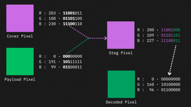
Tools like JSteg help hide data within the DCT coefficients of a JPEG image. Checkout this video from Computerphile which gives an overview of this method. Then there are techniques such as PVD Steganography, HUGO (Highly Undetectable steGO), J-UNIWARD, S-UNIWARD etc. While these techniques ensure that no one ever finds even the slightest trace of hidden data, the downside is the limited payload capacity. These methods typically manage just 1-4 bpp (bits per pixel). The LSB steganography example shown above stores the image pixel data at 3bpp (As the first 3 most significant bits of the payload pixel are retained). There’s no way you’re hiding an image of a top-secret Area-51 UFO inside your Instagram DP with such low bit capacity!
But is it possible to encode all 8 bits of a payload pixel into a cover pixel? That would be 8 bits per channel × 3 channels (R,G,B) = 24 bpp. Seems like a very tough task to cook up an algorithm for this. But we know what the inputs and outputs are. Hmm, what do you do when you’ve got an impossible task at hand but know what the inputs and outputs are beforehand? Ahem, it’s time to add Neural Nets to the show.
Deep Image Steganography
One of the first works utilizing neural networks for this task is the paper Hiding Images in Plain Sight (2017) by S Baluja. Here, the author uses three sub-networks for image-in-image steganography. First, a prep network applies pre-processing to the input payload image, which is then concatenated with the cover image and passed on to a hiding network that generates the steganographic container image. The reveal network takes this container image to extract and decode the payload image. These three sub-networks are trained together in an end-to-end manner. This prep network can be helpful, especially in scenarios when the payload image has dimensions that differ from that of the cover image. Here, we’re exploring a simpler approach as described in this paper — just two sub-networks: an encoder to generate steganographic container images and a decoder to extract the embedded payload.
-
Encoder Network
The task of this network is to generate the steganographic container image. The input payload image is concatenated with the cover image to create a 6-channel tensor, which is then fed into the encoder (both images must have the same dimensions). This tensor passes through a series of convolution blocks with varying feature channel sizes (see the diagram). Each convolution block follows this structure: (a) convolution layer with a 3x3 kernel,zero padding and feature channels of size N=[3, 64, 128, 256, 512],(b) BatchNormalization layer, (c) ReLU activation layer, except for the last block, which uses a sigmoid activation. Another feature is the presence of concatenating skip connections between the initial and later convolution blocks of the encoder network.
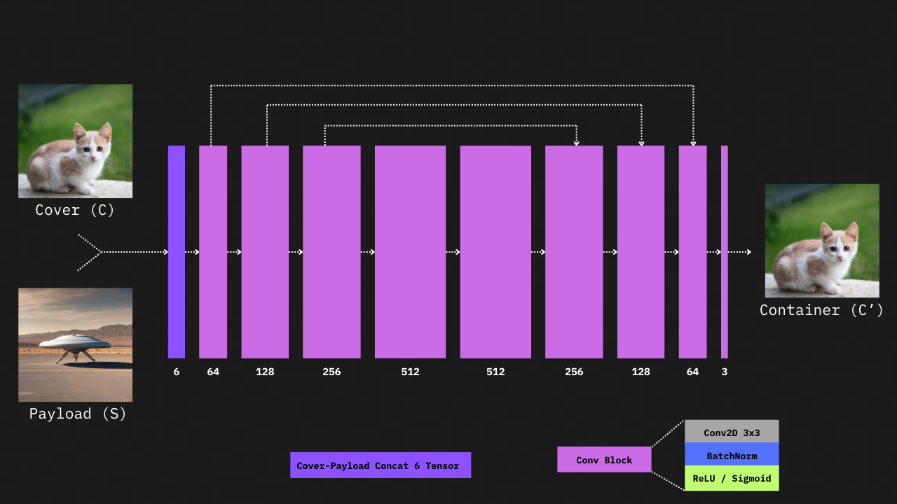 Encoder Network Architecture
-
Decoder Network
This network takes the steganographic container image and extracts the embedded payload image. It has the same structure as the encoder, but without the skip connections. Just like the encoder, this network has convolutional blocks with feature channels of N = [3, 64, 128, 256]. The last convolution block includes a 3-channel convolution layer, followed by a batch normalization layer and a sigmoid activation, to give an RGB output of the extracted payload image.
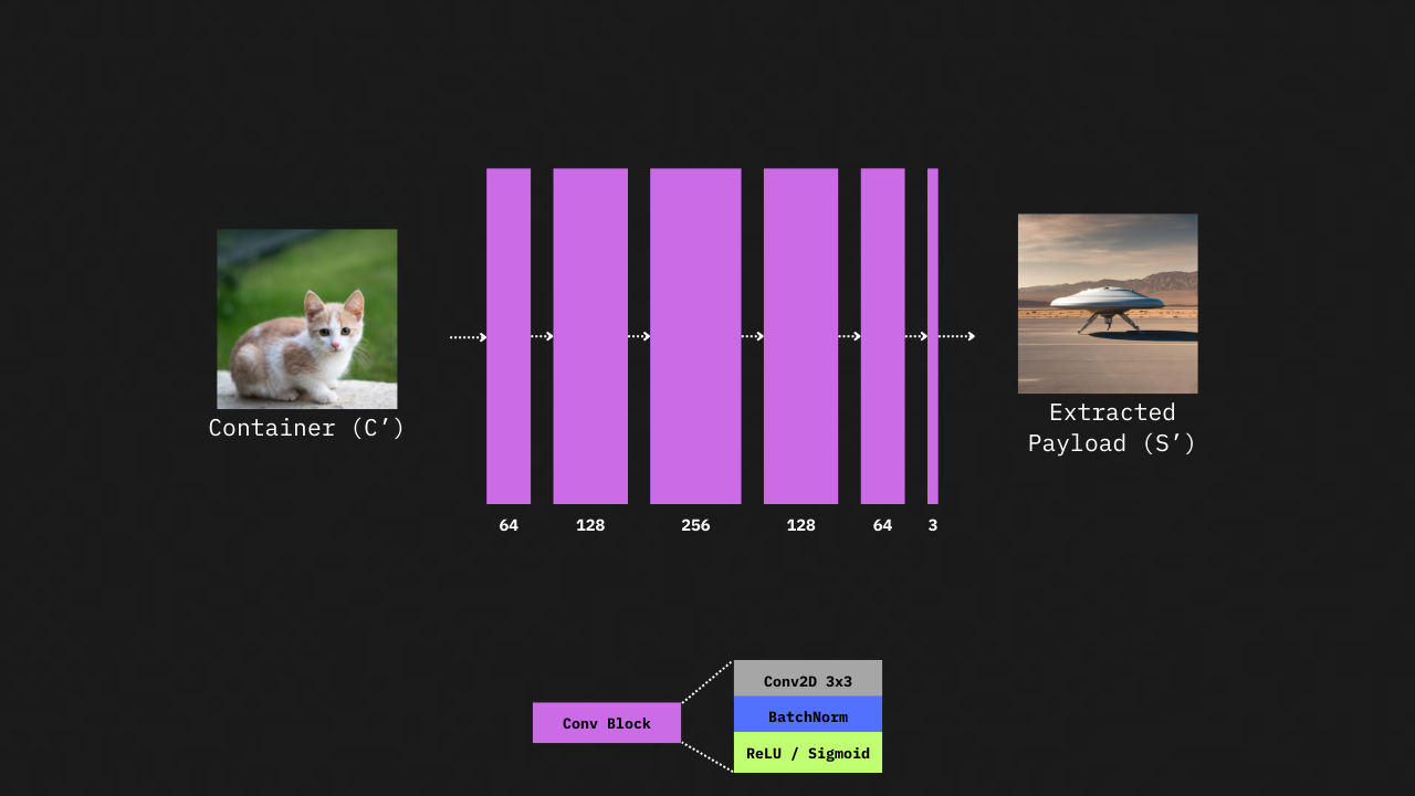 Decoder Network Architecture
These two networks are trained together in an end-to-end manner. As the combined network has two outputs (container image, extracted payload) we need to use a modified loss function:
where C is the cover image, C’ is the generated container image, S is the payload image, and S’ is the extracted payload image. MSE(C, C’) measures the error between the cover and container images, while MSE(S, S’) measures the error between the original and extracted payloads. The factor β adjusts how much weight each error gets. The Adam optimizer is used with a learning rate of 0.01 for training.
While the loss function trains the model, you also need to check how closely the generated container matches the original cover and how well the extracted payload matches the original. For this, we use metrics like PSNR and SSIM. PSNR (Peak Signal-to-Noise Ratio) measures the quality of the generated image compared to the original. Higher PSNR values indicate better quality and less distortion. It’s useful for assessing how closely the generated image matches the original image in terms of pixel values. SSIM (Structural Similarity Index) evaluates the visual similarity between two images by comparing their structure, luminance, and contrast. It gives a value between 0 and 1, where 1 means the images are identical. SSIM is more sensitive to changes in structural information compared to PSNR, making it a better measure for perceived visual quality.
For implementation you can check out the notebooks at github.com/Acedev003/Deep-Steganography.
Ending Notes
While this network can achieve 24 bpp in payload capacity, it’s far from perfect for any practical use. Besides the low resolution for both cover and payload (due to GPU memory and dataset limits), it also requires the cover and payload to be the same size. Plus, it’s not fully resistant to image file compression algorithms. Deep steganographic container images are good at concealing hidden info, but they can be vulnerable to adversarial attacks. These attacks make tiny changes that don’t affect the visual appearance but can completely mess up the hidden payload.
There are many tweaks that can make this network more practical and resistant to attacks, but that’s a topic for a later article. Until then, tschüss!
References
- Baluja, S.: Hiding Images in Plain Sight: Deep Steganography. In: Advances in Neural Information Processing Systems. Curran Associates, Inc. (2017)
- Kich, I.: Image Steganography by Deep CNN Auto-Encoder Networks. IJATCSE. 9, 4707–4716 (2020). https://doi.org/10.30534/ijatcse/2020/75942020